Introduction to pixieweb

pixieweb is an R package for discovering, inspecting and downloading statistical data from PX-Web APIs — the platform used by Statistics Sweden (SCB), Statistics Norway (SSB), Statistics Finland, and many other national statistics agencies. This vignette provides an overview of the methods included in the pixieweb package and the design principles of the package API. To learn more about the specifics of functions and to see a full list of the functions included, please see the Reference section of the package homepage or run ??pixieweb. For a quick introduction to the package see the vignette Quick start guide to pixieweb.

Note on pxweb: The excellent pxweb package by rOpenGov already provides comprehensive R access to PX-Web APIs. pixieweb is not a replacement — it offers an alternative paradigm built around search-then-fetch discovery and progressive disclosure. Choose the workflow that fits your needs.

The design of pixieweb functions is inspired by the design and functionality provided by several packages in the tidyverse family. pixieweb uses the base R pipe (|>) throughout. Some vignette examples use dplyr, tidyr, and ggplot2 for data wrangling and visualisation:

install.packages("pixieweb")

PX-Web, a platform for national statistical databases

PX-Web is the statistical database platform used by national statistics agencies across the Nordic countries and beyond. Each agency runs its own instance — Statistics Sweden at scb.se, Statistics Norway at ssb.no, Statistics Finland at stat.fi, and many more — but they all share the same underlying API, which comes in two versions:

• v1 — the legacy API, still widely deployed. POST-only data queries, no search endpoint, table discovery requires walking a folder hierarchy.
• v2 — the modern API, launched by SCB in 2024. GET+POST data queries, full-text search, codelists endpoint, server-side saved queries.

pixieweb handles both versions transparently — the user-facing functions have the same signatures, and only the internal request building differs.

To get started with PX-Web you might want to visit the web frontend of any participating agency, or read through the PxWebApi2 documentation (English). However, you can also use the pixieweb package to explore data without prior knowledge of the database.

library("pixieweb")

The data model

Data in PX-Web are stored as multi-dimensional data cubes. Each agency publishes hundreds or thousands of tables, and each table defines its own set of variables (dimensions) along which observations are indexed. A typical population table might, for instance, be indexed by region, sex, age and year — while a foreign trade table might be indexed by partner country, commodity group and month.

When downloading data, the user needs to specify which values to include along each variable — or omit the variable entirely, in which case the API returns a pre-computed aggregate (this is called elimination). Every table has its own rules for which variables are mandatory and which are eliminable.

In summary, a PX-Web table is organised along four basic concepts:

• An API instance — a particular agency’s PX-Web database (e.g. SCB, SSB)
• A table — a single statistical data cube published by that agency
• A set of variables — the dimensions of the cube (region, time, sex, product, etc.); each variable has a set of valid values
• One or more content codes — what is actually being measured in each cell (population count, deaths, tax revenue, GDP, …)

Tables with multiple content codes can return data in either long format (one row per observation, one column for the content code) or wide format (one column per content code) — see the section on wide output below.

Additionally, many variables come with one or more codelists — alternative groupings of the values that can be used to aggregate data on the fly. For example, a “Region” variable with 290 municipalities might offer codelists that group them into 21 counties, or into eight NUTS-2 regions.

pixieweb provides a function family for each of these concepts:

Level	Discover	Search	Describe	Extract	Values
API instance	px_api_catalogue()	—	—	—	—
Table	get_tables()	table_search()	table_describe()	table_extract_ids()	—
Variable	get_variables()	variable_search()	variable_describe()	variable_extract_ids()	variable_values()
Codelist	get_codelists()	—	codelist_describe()	codelist_extract_ids()	codelist_values()
Data	get_data()	—	—	—	—

Connecting to an API

All pixieweb workflows start by connecting to a PX-Web instance. px_api() accepts a short alias ("scb", "ssb", "statfi", …) or a full URL:

# Known aliases
scb <- px_api("scb", lang = "en")
ssb <- px_api("ssb", lang = "en")

# Or a custom URL
custom <- px_api("https://my.statbank.example/api/v2/", lang = "en")

# See all known APIs
px_api_catalogue()

#> # A tibble: 13 × 7
#>    alias    description                 url   url_v1 versions langs default_lang
#>    <chr>    <chr>                       <chr> <chr>  <list>   <lis> <chr>       
#>  1 scb      Statistics Sweden (SCB)     http… https… <chr>    <chr> sv          
#>  2 ssb      Statistics Norway (SSB)     http… https… <chr>    <chr> no          
#>  3 statfi   Statistics Finland          http… https… <chr>    <chr> fi          
#>  4 statis   Statistics Iceland          http… https… <chr>    <chr> en          
#>  5 hagstova Statistics Faroe Islands    http… https… <chr>    <chr> fo          
#>  6 statgl   Statistics Greenland        http… https… <chr>    <chr> da          
#>  7 asub     Statistics Åland (ÅSUB)     http… https… <chr>    <chr> sv          
#>  8 sjv      Swedish Board of Agricultu… http… https… <chr>    <chr> sv          
#>  9 energi   Swedish Energy Agency (Ene… http… https… <chr>    <chr> sv          
#> 10 fohm     Public Health Agency of Sw… http… https… <chr>    <chr> sv          
#> 11 konj     National Institute of Econ… http… https… <chr>    <chr> sv          
#> 12 msb      Swedish Civil Contingencie… http… https… <chr>    <chr> sv          
#> 13 slu      Swedish University of Agri… http… https… <chr>    <chr> sv

For cross-country comparison and a fuller tour of the multi-API catalogue, see vignette("multi-api").

Discovering tables: get_tables()

Tables are the central entity. On v2 APIs, get_tables() sends a server-side search query; on v1 APIs, it walks the folder tree. In both cases the result is a tibble with rich metadata, one row per table:

# Search the SCB catalogue for population-related tables
tables <- get_tables(scb, query = "population")

head(tables)

#> # A tibble: 6 × 13
#>   id      title  description category updated first_period last_period time_unit
#>   <chr>   <chr>  <chr>       <chr>    <chr>   <chr>        <chr>       <chr>    
#> 1 TAB638  Popul… ""          public   2025-0… 1968         2024        Annual   
#> 2 TAB1743 Incom… ""          public   2015-1… 1995         2013        Annual   
#> 3 TAB934  Famil… ""          public   2015-1… 1995         2013        Annual   
#> 4 TAB4552 Popul… ""          public   2025-0… 1960         2023        Annual   
#> 5 TAB6473 Popul… ""          public   2026-0… 2025M01      2026M01     Monthly  
#> 6 TAB1625 Popul… ""          public   2025-0… 2000M01      2024M12     Monthly  
#> # ℹ 5 more variables: variables <list>, subject_code <chr>, subject_path <chr>,
#> #   source <chr>, discontinued <lgl>

The table tibble includes subject path, time period range, time unit, and data source — all of which are searchable by table_search() (a client-side filter, analogous to kpi_search() in rKolada).

# Narrow down to tables about municipalities
tables |>
  table_search("municipal") |>
  table_describe(max_n = 2, format = "md", heading_level = 4)
#> Warning: No tables to describe.

table_describe() prints a human-readable summary of each table. As with all describe functions in the pixieweb/rKolada/rTrafa family, you can set format = "md" to produce Markdown output that can be embedded directly in an R Markdown document by setting the chunk option results = 'asis'.

Exploring variables: get_variables()

Once you have chosen a table, inspect its variables with get_variables():

vars <- get_variables(scb, "TAB638")
vars |> variable_describe()

#> ── Region (region) ────────────────────────────────────────────────────────────── 
#>   Values: 312, optional (elimination) 
#>   First values: 00 Sweden, 01 Stockholm county, 0114 Upplands Väsby, 0115 Vallentuna, 0117 Österåker ... and 307 more 
#>   Codelists: agg_RegionA-region_2 A-regions, agg_RegionLA1998 Local labour markets 1998, agg_RegionLA2003_1 Local labour markets 2003 ... and 15 more 
#> 
#> ── Civilstand (marital status) ────────────────────────────────────────────────── 
#>   Values: 4, optional (elimination) 
#>   First values: OG single, G married, ÄNKL widowers/widows, SK divorced 
#> 
#> ── Alder (age) ────────────────────────────────────────────────────────────────── 
#>   Values: 102, optional (elimination) 
#>   First values: 0 0 years, 1 1 year, 2 2 years, 3 3 years, 4 4 years ... and 97 more 
#>   Codelists: agg_Ålder10årJ ´10-year intervals, agg_Ålder5år 5-year intervals, vs_Ålder1årA Age, 1 year age classes ... and 1 more 
#> 
#> ── Kon (sex) ──────────────────────────────────────────────────────────────────── 
#>   Values: 2, optional (elimination) 
#>   First values: 1 men, 2 women 
#> 
#> ── ContentsCode (observations) ────────────────────────────────────────────────── 
#>   Values: 2, mandatory 
#>   First values: BE0101N1 Population, BE0101N2 Population growth 
#> 
#> ── Tid (year) ─────────────────────────────────────────────────────────────────── 
#>   Values: 57, mandatory 
#>   Time variable: Yes
#>   First values: 1968 1968, 1969 1969, 1970 1970, 1971 1971, 1972 1972 ... and 52 more

Each variable has a number of important properties worth knowing about:

• elimination — can this variable be left out of your get_data() call? If TRUE, omitting the variable means the API returns a pre-computed total (e.g. omitting “Sex” gives the total for all sexes). If FALSE, the variable is mandatory and must be included in the query.
• time — is this the time dimension of the cube? (There is always exactly one.)
• values — the set of available codes and their human-readable labels.
• codelists — alternative groupings of the values (see the “Codelists” section below).

To inspect the available values for a specific variable, use variable_values():

vars |> variable_values("Region")

#> # A tibble: 312 × 2
#>    code  text            
#>    <chr> <chr>           
#>  1 00    Sweden          
#>  2 01    Stockholm county
#>  3 0114  Upplands Väsby  
#>  4 0115  Vallentuna      
#>  5 0117  Österåker       
#>  6 0120  Värmdö          
#>  7 0123  Järfälla        
#>  8 0125  Ekerö           
#>  9 0126  Huddinge        
#> 10 0127  Botkyrka        
#> # ℹ 302 more rows

Downloading data: get_data()

get_data() is the workhorse function. Provide an API object, a table ID, and one argument per variable you want to include in the query:

pop <- get_data(scb, "TAB638",
  Region = c("0180", "1480", "1280"),
  ContentsCode = "*",
  Tid = px_top(5)
)

head(pop)

#> # A tibble: 6 × 8
#>   table_id Region Region_text ContentsCode ContentsCode_text Tid   Tid_text
#>   <chr>    <chr>  <chr>       <chr>        <chr>             <chr> <chr>   
#> 1 TAB638   0180   Stockholm   BE0101N1     Population        2020  2020    
#> 2 TAB638   0180   Stockholm   BE0101N1     Population        2021  2021    
#> 3 TAB638   0180   Stockholm   BE0101N1     Population        2022  2022    
#> 4 TAB638   0180   Stockholm   BE0101N1     Population        2023  2023    
#> 5 TAB638   0180   Stockholm   BE0101N1     Population        2024  2024    
#> 6 TAB638   0180   Stockholm   BE0101N2     Population growth 2020  2020    
#> # ℹ 1 more variable: value <dbl>

Variables you omit are eliminated (aggregated) if the API allows it. If a variable is mandatory, you must include it — get_data() will raise an informative error otherwise.

Selection helpers

Often you don’t want to hardcode specific codes. pixieweb provides a family of selection helpers that translate common wishes into API-compatible arguments:

Helper	Meaning	API versions
c("0180")	Specific values	v1, v2
"*"	All values	v1, v2
px_top(5)	First N values (e.g. most recent)	v1, v2
px_bottom(3)	Last N values	v2 only
px_from("2020")	From value onward	v2 only
px_to("2023")	Up to value	v2 only
px_range(a, b)	Inclusive range	v2 only

Metadata-driven queries: prepare_query()

An alternative approach to downloading data using known codes is to use the metadata tables to construct queries. For interactive exploration, prepare_query() inspects the table’s variable metadata and builds a query with sensible defaults, so that you only need to specify the variables you care about:

q <- prepare_query(scb, "TAB638",
  Region = c("0180", "1480", "1280")
)
q

#> ── Query: TAB638 ──────────────────────────────────────────────────────────────── 
#>   Estimated cells: 60 / 150000 (0% of limit)
#> 
#>   Region = c("0180", "1480", "1280")
#>     user override
#>   Civilstand = <eliminated>
#>     eliminated (4 values available)
#>   Alder = <eliminated>
#>     eliminated (102 values available)
#>   Kon = <eliminated>
#>     eliminated (2 values available)
#>   ContentsCode = "*"
#>     all 2 content variable(s)
#>   Tid = px_top(10)
#>     latest 10 of 57 periods

The default strategy is:

• Content code: all values ("*")
• Time variable: latest 10 periods (px_top(10))
• Eliminable variables: omitted (API aggregates)
• Small mandatory variables (≤ 22 values): all ("*")
• Large mandatory variables: first value (px_top(1))

With maximize_selection = TRUE, the function expands unspecified variables to include as many values as possible while staying under the API’s cell limit. Once you’re happy, pass the validated query to get_data():

pop <- get_data(scb, query = q)

Codelists

Codelists provide alternative groupings of variable values. They are useful when you want data at a different aggregation level than the table’s default. For example, a “Region” variable with 290 Swedish municipalities might have a codelist that groups them into 21 counties (vs_RegionLän07):

cls <- get_codelists(scb, "TAB638", "Region")
cls |> codelist_describe(max_n = 3)

#> ── agg_RegionA-region_2: A-regions ────────────────────────────────────────────── 
#>   Type: Aggregation 
#>   Values: 70 items 
#>   First: A-01 Stockholms/Södertälje A-region, A-02 Norrtälje A-region, A-03 Enköpings A-region, A-04 Uppsala A-region, A-05 Nyköpings A-region ... and 65 more 
#> 
#> ── agg_RegionLA1998: Local labour markets 1998 ────────────────────────────────── 
#>   Type: Aggregation 
#>   Values: 100 items 
#>   First: 01001LA Stockholm LA, 04001LA Nyköping-Oxelösund LA, 04002LA Katrineholm LA, 04003LA Eskilstuna LA, 05001LA Linköping LA ... and 95 more 
#> 
#> ── agg_RegionLA2003_1: Local labour markets 2003 ──────────────────────────────── 
#>   Type: Aggregation 
#>   Values: 87 items 
#>   First: LA0301 Stockholm LA, LA0302 Nyköping-Oxelösund LA, LA0303 Eskilstuna LA, LA0304 Linköping LA, LA0305 Norrköping LA ... and 82 more

Apply a codelist in a query via the .codelist argument:

# Fetch data aggregated to counties instead of municipalities
get_data(scb, "TAB638",
  Region = "*",
  Tid = px_top(5),
  ContentsCode = "*",
  .codelist = list(Region = "vs_RegionLän07")
)

Wide output and multiple content codes

When a table has multiple content codes (e.g. both Population and Deaths), the default long format has one row per content code per observation. Use .output = "wide" to pivot the content codes into separate columns — useful when you want to compute with several measures (e.g. death rate = Deaths / Population):

demo <- get_data(scb, "TAB638",
  Region = "0180",
  Tid = px_top(5),
  ContentsCode = "*",
  .output = "wide"
)
demo

#> # A tibble: 5 × 7
#>   table_id Region Region_text Tid   Tid_text BE0101N1 BE0101N2
#>   <chr>    <chr>  <chr>       <chr> <chr>       <dbl>    <dbl>
#> 1 TAB638   0180   Stockholm   2020  2020       975551     1477
#> 2 TAB638   0180   Stockholm   2021  2021       978770     3219
#> 3 TAB638   0180   Stockholm   2022  2022       984748     5978
#> 4 TAB638   0180   Stockholm   2023  2023       988943     4195
#> 5 TAB638   0180   Stockholm   2024  2024       995574     6631

Visualising results

To explore results we can plot the downloaded data using ggplot2. Note that we convert the time column to a Date first — years as integer can produce awkward ggplot breaks like “2020, 2022.5, 2025”, and a proper Date column lets scale_x_date() place tick marks on whole years. This is a pattern you will want to use for any time-series analysis across all three sibling packages (rKolada, pixieweb, rTrafa):

library("ggplot2")

pop_plot <- pop |>
  # Keep only the Population content code (the table also has
  # "Population growth"); convert year to Date for nice axis breaks
  dplyr::filter(ContentsCode == "BE0101N1") |>
  dplyr::mutate(year = as.Date(paste0(Tid, "-01-01")))

ggplot(pop_plot, aes(year, value, colour = Region_text)) +
  # One line per region; linetype adds distinction in B/W print
  geom_line(aes(linetype = Region_text), linewidth = 1) +
  geom_point(size = 2) +
  # Years as dates, one tick per year
  scale_x_date(date_breaks = "1 year", date_labels = "%Y") +
  scale_y_continuous(labels = scales::comma) +
  # Colour-blind-friendly palette
  scale_colour_viridis_d(option = "B", end = 0.8) +
  labs(
    title = "Population, Sweden's three most populous municipalities",
    x = "Year",
    y = "Population",
    colour = NULL,
    linetype = NULL,
    caption = px_cite(pop)
  ) +
  theme_minimal() +
  theme(legend.position = "top")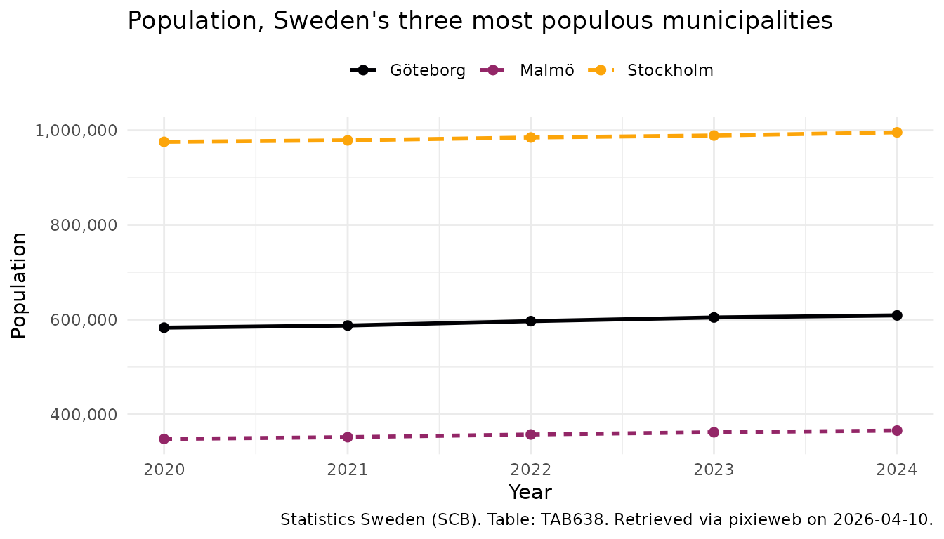

More on ggplot2? See https://ggplot2-book.org/.

Advanced: query composition

For full control over the HTTP request — useful for debugging or when you need to inspect/modify the exact query before sending it — use the low-level query composers:

q <- compose_data_query(scb, "TAB638",
  Region = c("0180"),
  ContentsCode = "*",
  Tid = px_top(3)
)

# Inspect the query
q$url
q$body

# Modify and execute
raw <- execute_query(scb, q$url, q$body)

Saved queries (v2 only)

PX-Web v2 supports server-side stored queries — useful for recurring reports. Save a query once, then retrieve it by ID later:

# Save a query
id <- save_query(scb, "TAB638",
  Region = "0180",
  Tid = px_top(5),
  ContentsCode = "*"
)

# Retrieve later
get_saved_query(scb, id)

Citation

Always cite your data sources. px_cite() generates a citation string from the metadata attached to a downloaded data frame:

px_cite(pop)

#> [1] "Statistics Sweden (SCB). Table: TAB638. Retrieved via pixieweb on 2026-04-10."

Related packages

pixieweb is part of a family of R packages for Swedish and Nordic open statistics that share the same design philosophy:

• rKolada — R client for the Kolada database of Swedish municipal and regional Key Performance Indicators
• rTrafa — R client for the Trafa API of Swedish transport statistics

See also pxweb — the original and established PX-Web client for R, by rOpenGov.